

Identify the normal and intrinsic curves
A demagnetization curve shows the magnet's behaviour as an opposing magnetic field is applied after magnetization. Start with the second quadrant: H is negative while the plotted B or J remains positive over the useful part of the branch. Identify the plotted quantity before reading any intercept or operating point.[1] [3]
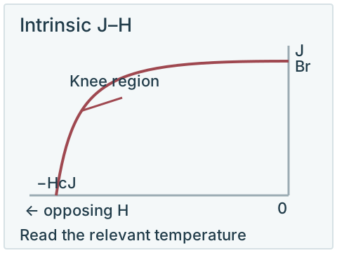
The normal curve plots flux density B against field H. The intrinsic curve plots magnetic polarization J against H; some documents use an intrinsic-induction notation instead. In SI, B = μ₀H + J. At H = 0 the two branches share the remanent value, but away from that point they represent different vertical quantities. A legacy-unit chart needs its own axis conventions checked.[1] [6]
The cover separates the two plots deliberately. “Magnetization curve” can also refer to an initial magnetization curve or a full hysteresis loop. Confirm which document is intended; this guide covers the demagnetization branch, not every part of a full loop.
Read the characteristic points
| Parameter | Where to read it | What to avoid |
|---|---|---|
| Br | The remanent value at H = 0 after magnetization. | Treating it as the surface field of any finished shape. |
| HcB | The magnitude of the opposing field at B = 0 on the normal curve. | Reading the intrinsic intercept instead. |
| HcJ | The magnitude of the opposing field at J = 0 on the intrinsic curve. | Assuming it is the same quantity as HcB. |
| (BH)max | The greatest magnitude of B × H along the normal second-quadrant branch. | Multiplying Br by HcJ or treating energy density as pull force. |
Read each parameter from the correct curve
Br
- Where to read it
- The remanent value at H = 0 after magnetization.
- What to avoid
- Treating it as the surface field of any finished shape.
HcB
- Where to read it
- The magnitude of the opposing field at B = 0 on the normal curve.
- What to avoid
- Reading the intrinsic intercept instead.
HcJ
- Where to read it
- The magnitude of the opposing field at J = 0 on the intrinsic curve.
- What to avoid
- Assuming it is the same quantity as HcB.
(BH)max
- Where to read it
- The greatest magnitude of B × H along the normal second-quadrant branch.
- What to avoid
- Multiplying Br by HcJ or treating energy density as pull force.
A rectangular B × H area can illustrate energy product at a point on the normal curve. The largest such magnitude is (BH)max. It is a material comparison quantity, not proof that the assembly operates at that point. Property tables and curve axes must use a consistent unit system.[1] [6]
The property guide explains the quantities, while the datasheet checklist helps retain the supplier, grade, temperature and revision behind them.
Locate the operating point for the magnetic circuit
For a simplified magnetic-circuit representation, the intersection of the normal B–H curve and the circuit's load line identifies an operating point. The circuit includes the magnet geometry, return path and air gaps. Altering those conditions can move the intersection even though the material grade remains unchanged.[2] [3]
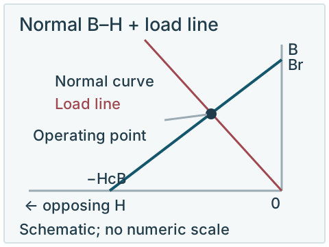
The permeance coefficient Pc expresses the operating relationship using the definition and units adopted by the reference. Keep those conventions with the value. There is no single Pc number that proves every magnet, temperature and opposing-field condition is safe.
Two changes to compare on the same normal curve
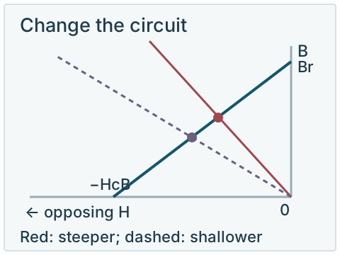
For an idealized circuit with no applied opposing excitation, consider a straight load line through the origin. With the material and temperature fixed, a steeper negative slope intersects the normal curve closer to H = 0, at a higher B. A shallower negative slope moves the intersection toward more negative H and lower B. Actual slope changes depend on the magnet and return path, not a shape name alone.
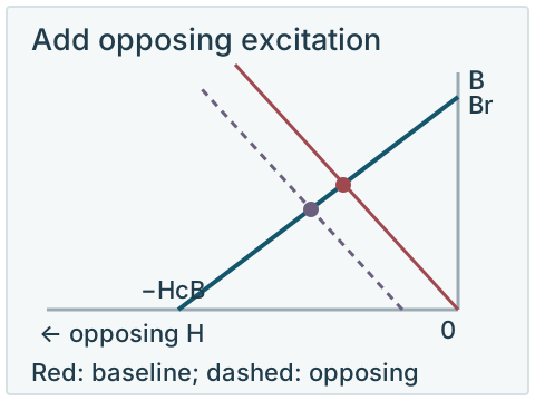
Now hold the geometry fixed and add an opposing excitation. In the simplified motor model in the ORNL report, the load line shifts left without changing slope. This moves the operating point farther down the same curve. Changing the circuit geometry and adding an opposing field are therefore different changes; they should not be illustrated as the same operation.[2]
Changing temperature is a third comparison: use the material's curve at that temperature and check its intersection with the applicable load line. If an excursion crosses the relevant knee, returning the excitation or temperature does not necessarily restore the original magnetic state. These are qualitative reading examples, with no numeric material data or predicted loss.
The load line in this illustration belongs to the normal B–H panel. Applying the same line to an intrinsic J–H panel and calling its intersection the same operating point would mix different quantities. Supplier calculators can help explore assumed shapes and conditions, but their output needs to be understood within the stated model.[4]
Check the curve at the relevant temperature
Read the curve for the specified grade at the temperature of interest. As the curve shape changes, the operating point and any opposing-field excursion need to be checked against the knee and the acceptable permanent loss. A room-temperature curve plus a maximum-temperature label does not establish that margin for an actual assembly.[2] [3] [5]
Provide the geometry, circuit, temperature duty and opposing-field conditions for the evaluation. In a motor application, the relevant operating and fault conditions are specific to the design. See temperature-related losses, grade suffixes and the high-temperature inquiry checklist for the connected requirements.
If you need numerical curve data
Request supplier-issued data with the grade, temperature, axis quantities, units, measurement or modelling conditions, revision and permitted use. Identify whether you need measured data or a supplier's model. The conceptual diagrams here have no numerical scale and cannot serve as a material CSV or simulation input.
Explore this requirement
Technical sources
Read each source with its stated material, test conditions and publication scope.
- NdFeB Standard Grade Data Sheet
- Fessler (2011), Assessment of Motor Technologies for Traction Drives of Hybrid and Electric VehiclesORNL/TM-2011/73. PDF pp. 22–23 (printed pp. 9–10): load line and operating point; PDF p. 34 (printed p. 21): demagnetization design tradeoffs.
- Magnetic Circuit Design Guide
- BH Curves Calculator
- Demagnetization Curve Explained
- Arnold Neo CatalogHistorical catalogue: field and curve-reading examples, not current purchasing data.