

What α and β mean
A temperature coefficient estimates how much a specified magnetic property changes per degree over a stated temperature range. NdFeB data sheets commonly give separate coefficients for remanence and intrinsic coercivity.
α describes the change in remanence Br, the flux-density value at zero applied field on the material's demagnetization curve.
β commonly describes the change in intrinsic coercivity HcJ, a measure related to resistance to demagnetization. HcJ is also written Hci; it is the reverse field where intrinsic polarization reaches zero. [1]
| Entry | Meaning | Reading the data |
|---|---|---|
| α(Br) | Change in the material's remanence | Describes Br, rather than surface field or assembly pull force |
| β(HcJ) or β(Hci) | Change in intrinsic coercivity | Keep HcJ separate from HcB, the coercivity of the normal B–H curve |
| %/°C | Relative percentage change per Celsius degree | For example, −0.12 %/°C equals −0.0012 per °C |
| Applicable interval | The range over which the stated coefficient is used | Check separately from the maximum operating-temperature rating |
Temperature-coefficient notation
α(Br)
- Meaning
- Change in the material's remanence
- Reading the data
- Describes Br, rather than surface field or assembly pull force
β(HcJ) or β(Hci)
- Meaning
- Change in intrinsic coercivity
- Reading the data
- Keep HcJ separate from HcB, the coercivity of the normal B–H curve
%/°C
- Meaning
- Relative percentage change per Celsius degree
- Reading the data
- For example, −0.12 %/°C equals −0.0012 per °C
Applicable interval
- Meaning
- The range over which the stated coefficient is used
- Reading the data
- Check separately from the maximum operating-temperature rating
Published coefficients and temperature ranges
Use the coefficients supplied for your material. The examples below come from separate specifications. Bakker prints the minus sign in its column heading; it is included with each value here.
| Source and grade | α(Br), %/°C | β(HcJ/Hci), %/°C | Temperature interval and basis |
|---|---|---|---|
| SM Magnetics, N35 [1] | −0.12 | −0.60 | Coefficient interval not stated on the cited page; request it before application |
| Bakker, N35SH/ST [3] | −0.115 | −0.62 | 20 to 100 °C; typical values, December 2025 sheet |
| Bakker, N35SH/ST [3] | −0.12 | −0.56 | 20 to 150 °C; typical values, same sheet |
Examples of published NdFeB coefficient data, checked 31 October 2026
SM Magnetics, N35 [1]
- α(Br), %/°C
- −0.12
- β(HcJ/Hci), %/°C
- −0.60
- Temperature interval and basis
- Coefficient interval not stated on the cited page; request it before application
Bakker, N35SH/ST [3]
- α(Br), %/°C
- −0.115
- β(HcJ/Hci), %/°C
- −0.62
- Temperature interval and basis
- 20 to 100 °C; typical values, December 2025 sheet
Bakker, N35SH/ST [3]
- α(Br), %/°C
- −0.12
- β(HcJ/Hci), %/°C
- −0.56
- Temperature interval and basis
- 20 to 150 °C; typical values, same sheet
Bakker gives different coefficients for the same grade over two intervals. Record the supplier, grade, document revision and temperature interval with each value. Request missing data from that material's supplier before calculating.
Calculation and worked examples
Use a coefficient whose definition and interval suit the starting property value. For a signed numerical coefficient c in %/°C:
X(T) ≈ X(T₀) × [1 + c × (T − T₀) / 100]
X is Br or HcJ; use its matching coefficient c (α or β). T₀ is the reference temperature and T is the temperature being evaluated, both in °C. X(T₀) is the starting property value.
Here c is the signed numerical value in %/°C. If it has already been converted to a decimal per °C, omit the division by 100.
This linear approximation is a preliminary material calculation. Follow the source's convention if it defines the coefficient differently. [4]
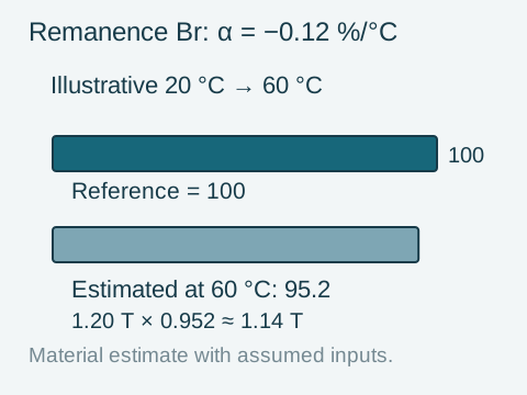
Worked example: Br from 20 °C to 60 °C
For this arithmetic example, assume Br(20 °C) = 1.20 T and α = −0.12 %/°C applicable over the full interval. These inputs illustrate the method and do not identify a supplied grade.
- Temperature rise: 60 − 20 = 40 °C.
- Relative change: −0.12 × 40 = −4.8%.
- Remaining fraction: 1 − 4.8/100 = 0.952.
- Calculation: 1.20 × 0.952 = 1.1424 T, reported here as about 1.14 T.
The extra arithmetic digits do not indicate measurement accuracy.
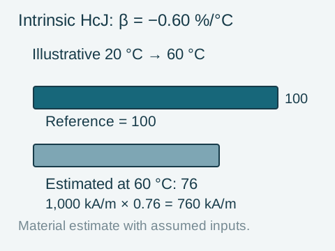
Worked example: intrinsic coercivity
Assume HcJ(20 °C) = 1,000 kA/m and β = −0.60 %/°C, also valid over the chosen 40 °C rise. The estimated relative change is −24%, giving HcJ(60 °C) ≈ 760 kA/m. Whether that value is sufficient depends on the operating point and opposing field in the design.
A temperature difference of 1 K has the same size as a difference of 1 °C. Convert Fahrenheit temperatures to Celsius before using a coefficient per Celsius degree.
Using the result in an assembly
For a holding assembly, calculate or test the force with its actual target, gap and geometry at the relevant temperature. Br is one material input. Its percentage change cannot be applied directly to the holding-force rating. [4]
For a sensor, compare the field at the sensing position with the sensor's permitted range. In either case, keep the fixture and measurement location fixed when comparing temperatures, and account for changes in the assembly where relevant.
Will the magnet recover after cooling?
A reversible change recovers when the magnet returns to its reference temperature. Irreversible demagnetization leaves a loss after cooling. Temperature coefficients alone cannot predict which will occur. [5]
That assessment uses temperature-dependent demagnetization curves, the circuit load line and opposing fields. Geometry and the magnetic return path affect the working point: K&J's examples show how the same material can behave differently in different circuits. [6]
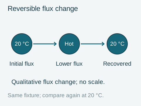
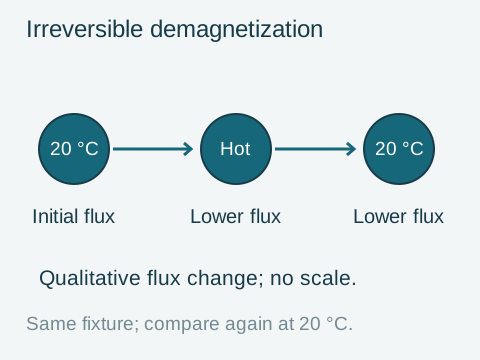
If a test shows lower flux after cooling, investigate the cause before assigning it to demagnetization. The diagrams show qualitative flux changes; they do not use the Br or HcJ percentages calculated above.
For a test specification, distinguish the output required while hot from the permitted loss after cooling. The demagnetization-curve guide explains the curve quantities; temperature limits covers operating conditions. Curie temperature is a separate material transition.
Calculation checks
- Use the coefficient for the stated property, grade and document.
- Check that both reference and target temperatures lie within the coefficient's applicable interval, and convert percent once.
- Keep units with the result and label it as an estimate, specified limit or measurement.
Ask about a temperature coefficient
Send the data sheet and the temperature you need to evaluate, with the entry or calculation that is unclear. For a component enquiry, include the drawing, temperature range and duration of exposure.
Temperature-data question
Supplier / grade and source document:
Reference temperature and target temperature:
Property or calculation to check:
Missing value or question:
For a complete application assessment
Add temperature-dependent curves, geometry, magnetic circuit and opposing fields, required output while hot, and permitted loss after cooling. A coefficient calculation by itself does not establish those acceptance conditions.
Technical sources
- SM Magnetics / SuperMagnetMan: Neodymium Material SpecsN35 material data, including the published Br and Hci temperature coefficients.
- Dura Magnetics: Available Neodymium Magnet Grades3512 / N35 grade properties and operating-temperature conditions. This table does not specify temperature coefficients or their applicable intervals.
- Bakker Magnetics: NdFeB corrosion and temperature stable gradesDecember 2025 data sheet: N35SH/ST typical coefficients for 20 to 100 °C and 20 to 150 °C; the minus sign appears in the column heading.
- Dura Magnetics: Does Temperature Affect the Strength of a Magnet?First-order temperature calculations and the limits of using Br to estimate assembly performance.
- Bunting: Temperature Coefficients of MagnetsDefinitions of temperature coefficients and reversible, irreversible and irrecoverable losses.
- K&J Magnetics: Temperature and neodymium magnetsSections 3 and 4: permeance coefficient, magnet geometry and temperature-dependent demagnetization curves.